cat articles/rapids-svr-svc-marc-ja

RAPIDS SVR and SVC: fast training without fine-tuning, evaluated on MARC-ja

created 2022-12-13

I learned about RAPIDS SVR and SVC in the Kaggle competition Feedback Prize - English Language Learning. They train quickly, and I felt they were useful methods for regression and classification tasks, so I will introduce what they are. In fact, top solutions in that competition used RAPIDS SVR.

I will also use RAPIDS SVC to evaluate MARC-ja, the classification dataset in the Japanese evaluation benchmark JGLUE. The implementation used for the evaluation is available on GitHub.

This article was written for day 13 of the Kaggle Advent Calendar 2022.

What are SVR and SVC?

SVR is Support Vector Regression, and SVC is Support Vector Classification. The algorithm behind them is SVM, or Support Vector Machine, which is known for strong accuracy and was apparently very popular at one point. sklearn also has an implementation, so many people have probably used it.

However, as the sklearn documentation says:

The implementation is based on libsvm. The fit time complexity is more than quadratic with the number of samples which makes it hard to scale to datasets with more than a couple of 10000 samples.

In other words, with sklearn's libsvm-based implementation, scaling past around ten thousand samples is not very realistic.

What are RAPIDS SVR and SVC?

RAPIDS SVR and SVC are SVM implementations in cuML, which is part of RAPIDS, NVIDIA's project for GPU-accelerated data science. Roughly speaking, cuML implements general-purpose machine learning algorithms similar to those in sklearn, follows sklearn's estimator API such as fit() and transform(), and optimizes them to run on CUDA. According to its benchmarks, it is 10 to 50 times faster than sklearn. That means algorithms that are difficult to run at practical speed in sklearn can become practical with cuML. RAPIDS also includes other CUDA-based tools, such as cuDF for fast DataFrame operations, so it is worth looking at the rest of the project if you are interested.

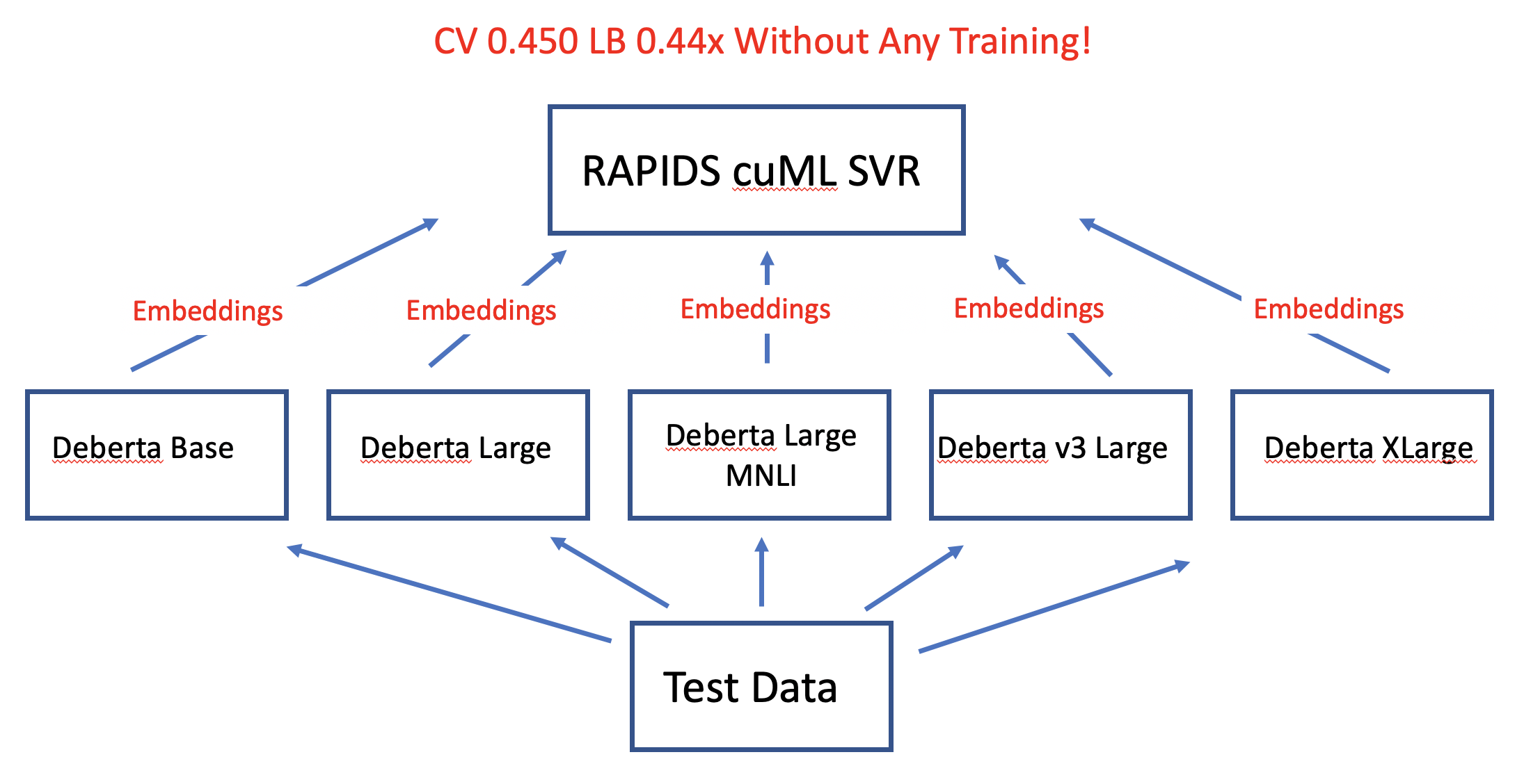
What becomes useful when SVR can run quickly? One answer is that training on the embedding representation from a neural network output layer becomes practical. You can take an existing public model, use it only for feature extraction without fine-tuning, and train SVR on those features. It is also easy to combine features from multiple models and train on the concatenated features. You can use non-fine-tuned models this way, but fine-tuned models can also be used as feature extractors.

RAPIDS SVR
--Quoted from RAPIDS SVR starter kit

Extracting features from neural networks

How should we extract features from a neural network? As an example, I will describe encoder models from Hugging Face Transformers. For most encoder models, you can either take the CLS token from last_hidden_state or apply mean pooling. The resulting vectors are then normalized before use.

class MeanPooling(nn.Module):
    def __init__(self, eps=1e-6):
        super(MeanPooling, self).__init__()
        self.eps = eps

    def forward(
        self, outputs: torch.Tensor, attention_mask: torch.Tensor
    ) -> torch.Tensor:
        last_hidden_state = outputs[0]
        input_mask_expanded = (
            attention_mask.unsqueeze(-1).expand(last_hidden_state.size()).float()
        )
        sum_embeddings = torch.sum(last_hidden_state * input_mask_expanded, 1)
        sum_mask = input_mask_expanded.sum(1)
        sum_mask = torch.clamp(sum_mask, min=self.eps)
        mean_embeddings = sum_embeddings / sum_mask
        return mean_embeddings

class ClsPooling(nn.Module):
    # 実際は Pooling ではなくただの CLS を取り出しているだけなので、このクラス名は良くない…
    def __init__(self):
        super(ClsPooling, self).__init__()

    def forward(
        self, outputs: torch.Tensor, attention_mask: torch.Tensor
    ) -> torch.Tensor:
        last_hidden_state = outputs[0]
        return last_hidden_state[:, 0, :]

POOLING_CLASSES = {
    "mean": MeanPooling,
    "cls": ClsPooling,
}

class TransformerEmbsModel(torch.nn.Module):
    def __init__(self, model_name: str, pooling: str = "mean"):
        super().__init__()
        self.model = AutoModel.from_pretrained(model_name)
        self.pool = POOLING_CLASSES[pooling]()

    def feature(self, inputs: dict[str, torch.Tensor]) -> torch.Tensor:
        outputs = self.model(**inputs)
        sentence_embeddings = self.pool(outputs, inputs["attention_mask"])
        # Normalize the embeddings
        sentence_embeddings = F.normalize(sentence_embeddings, p=2, dim=1)
        sentence_embeddings = sentence_embeddings.squeeze(0)
        return sentence_embeddings

    def forward(self, inputs: dict[str, torch.Tensor]) -> torch.Tensor:
        embs = self.feature(inputs)
        return embs

This is enough to extract features.

Training with RAPIDS SVC

After that, we only need to train with SVC. SVR works with almost the same code.

from cuml.svm import SVC
import numpy as np

DEFAULT_SVC_PARAMS = {
    "C": 3.0,  # Penalty parameter C of the error term.
    "kernel": "rbf",  # Possible options: ‘linear’, ‘poly’, ‘rbf’, ‘sigmoid’.
    "degree": 3,
    "gamma": "scale",  # auto or scale
    "coef0": 0.0,
    "tol": 0.001,  # 0.001 = 1e-3
}

def train_svc(
    X: np.ndarray,
    y: np.ndarray,
    svc_params: dict[str, object] = DEFAULT_SVC_PARAMS,
    probability: bool = True,
) -> SVC:
    svc = SVC(**svc_params)
    svc.probability = probability
    svc.fit(X, y)
    return svc

The core is almost just this.

Measuring the score on MARC-ja

Now let's evaluate MARC-ja, the classification dataset in the Japanese evaluation benchmark JGLUE. MARC-ja is a binary positive/negative sentiment classification dataset built from Japanese Amazon reviews. It has 187,528 train samples and 5,654 dev, or validation, samples. That is a reasonably large dataset. The test data does not seem to be publicly available at the moment.

JGLUE's GitHub page lists dev accuracy scores. For example, cl-tohoku/bert-base-japanese-v2 gets 0.958 after four epochs. The top score shown there is 0.964 from XLM-RoBERTa large.

Training time is also interesting. When I ran training casually on Colab with a T4 GPU, one epoch of bert-base-japanese-v2 took about 100 minutes, with 0.9573 accuracy after the first epoch. On my local RTX 4090, one epoch took about 30 minutes.

Feature extraction and SVC training

https://github.com/hotchpotch/rapids-svr-svc-marc_ja

In the repository above, I implemented feature extraction from a neural network on MARC-ja and training with RAPIDS SVC. Let's first train and evaluate SVC using cl-tohoku/bert-base-japanese-v2 without fine-tuning. The execution times below are from my local RTX 4090.

$ python lib/runner.py bert-base-ja-v2-cls
[create cache] tmp/embs_cache/bert-base-ja-v2-cls.pkl.gz
100%|███████████████████████████████████████████████████████████████████████| 5861/5861 [06:04<00:00, 16.09it/s]
100%|█████████████████████████████████████████████████████████████████████████| 177/177 [00:10<00:00, 16.45it/s]
exec time: 394.05 sec
shape: (187528, 768) (5654, 768)
concat embs: (187528, 768) (5654, 768)
[train svc]
svc exec time: 17.83 sec
==================================================
bert-base-ja-v2-cls
valid acc score: 0.927661832331093
==================================================
              precision    recall  f1-score   support

    positive    0.89788   0.56691   0.69500       822
    negative    0.93067   0.98903   0.95896      4832

    accuracy                        0.92766      5654
   macro avg    0.91428   0.77797   0.82698      5654
weighted avg    0.92590   0.92766   0.92059      5654

Feature extraction took 394 seconds, SVC training took about 18 seconds, and the accuracy was 0.92766. Once features are extracted, my implementation reuses them as a cache, so the second run costs almost only the SVC training time.

Next, let's look at the same model with mean pooling instead of CLS.

$ python lib/runner.py bert-base-ja-v2-mean
[load cache] tmp/embs_cache/bert-base-ja-v2-mean.pkl.gz
shape: (187528, 768) (5654, 768)
concat embs: (187528, 768) (5654, 768)
[train svc]
svc exec time: 18.44 sec
==================================================
bert-base-ja-v2-mean
valid acc score: 0.9324372125928546
==================================================
              precision    recall  f1-score   support

    positive    0.91667   0.58881   0.71704       822
    negative    0.93406   0.99089   0.96164      4832

    accuracy                        0.93244      5654
   macro avg    0.92536   0.78985   0.83934      5654
weighted avg    0.93153   0.93244   0.92608      5654

I had already run this before, so the features were loaded from cache and only SVC training was needed. Accuracy was 0.93244, so mean pooling worked better than CLS. What happens if we train on both sets of features?

$ python lib/runner.py bert-base-ja-v2-cls bert-base-ja-v2-mean
[load cache] tmp/embs_cache/bert-base-ja-v2-cls.pkl.gz
shape: (187528, 768) (5654, 768)
[load cache] tmp/embs_cache/bert-base-ja-v2-mean.pkl.gz
shape: (187528, 768) (5654, 768)
concat embs: (187528, 1536) (5654, 1536)
[train svc]
svc exec time: 30.04 sec
==================================================
bert-base-ja-v2-cls + bert-base-ja-v2-mean
valid acc score: 0.9334984082065794
==================================================
              precision    recall  f1-score   support

    positive    0.90545   0.60584   0.72595       822
    negative    0.93652   0.98924   0.96216      4832

    accuracy                        0.93350      5654
   macro avg    0.92099   0.79754   0.84405      5654
weighted avg    0.93200   0.93350   0.92782      5654

Because both feature sets were already cached, loading was almost instant, and SVC training took about 30 seconds. The result was 0.93350. Even with the same neural network model, extracting CLS and mean-pooled features separately and training on them together improved the score by about 0.001.

How about classic TF-IDF? TF-IDF features have too many dimensions as-is, so I reduced them to 1000 dimensions with SVD and then trained and evaluated SVC.

$ python lib/runner.py tfidf
[load cache] tmp/embs_cache/tfidf.pkl.gz
shape: (187528, 1000) (5654, 1000)
concat embs: (187528, 1000) (5654, 1000)
[train svc]
svc exec time: 55.78 sec
==================================================
tfidf
valid acc score: 0.8924655111425539
==================================================
              precision    recall  f1-score   support

    positive    0.81657   0.33577   0.47586       822
    negative    0.89729   0.98717   0.94009      4832

    accuracy                        0.89247      5654
   macro avg    0.85693   0.66147   0.70797      5654
weighted avg    0.88556   0.89247   0.87260      5654

Accuracy was 0.89247, which is not very good. For text with many unseen words, this is probably about what we should expect. Then what happens if we combine TF-IDF with BERT features?

$ python lib/runner.py bert-base-ja-v2-cls bert-base-ja-v2-mean tfidf
[load cache] tmp/embs_cache/bert-base-ja-v2-cls.pkl.gz
shape: (187528, 768) (5654, 768)
[load cache] tmp/embs_cache/bert-base-ja-v2-mean.pkl.gz
shape: (187528, 768) (5654, 768)
[load cache] tmp/embs_cache/tfidf.pkl.gz
shape: (187528, 1000) (5654, 1000)
concat embs: (187528, 2536) (5654, 2536)
[train svc]
svc exec time: 53.41 sec
==================================================
bert-base-ja-v2-cls + bert-base-ja-v2-mean + tfidf
valid acc score: 0.9379200565970994
==================================================
              precision    recall  f1-score   support

    positive    0.92280   0.62530   0.74547       822
    negative    0.93957   0.99110   0.96465      4832

    accuracy                        0.93792      5654
   macro avg    0.93119   0.80820   0.85506      5654
weighted avg    0.93713   0.93792   0.93278      5654

The result was 0.93792, much higher than BERT alone. TF-IDF points in a different direction as a feature source, so combining it likely added diversity and improved the score. It is also interesting that SVC training became slightly faster than TF-IDF alone, perhaps because convergence was better.

In the same way, I tried combining features from several Japanese models published on Hugging Face.

$ python lib/runner.py bert-base-ja-v2-cls bert-base-ja-v2-mean rinna-ja-roberta-base-cls rinna-ja-roberta-base-mean tfidf bert-base-ja-sentiment-cls bert-base-ja-sentiment-mean
[load cache] tmp/embs_cache/bert-base-ja-v2-cls.pkl.gz
shape: (187528, 768) (5654, 768)
...中略
[load cache] tmp/embs_cache/bert-base-ja-sentiment-mean.pkl.gz
shape: (187528, 768) (5654, 768)
concat embs: (187528, 5608) (5654, 5608)
[train svc]
svc exec time: 89.47 sec
==================================================
bert-base-ja-v2-cls + bert-base-ja-v2-mean + rinna-ja-roberta-base-cls + rinna-ja-roberta-base-mean + tfidf + bert-base-ja-sentiment-cls + bert-base-ja-sentiment-mean
valid acc score: 0.9432260346657234
==================================================
              precision    recall  f1-score   support

    positive    0.93717   0.65328   0.76989       822
    negative    0.94391   0.99255   0.96762      4832

    accuracy                        0.94323      5654
   macro avg    0.94054   0.82292   0.86876      5654
weighted avg    0.94293   0.94323   0.93887      5654

Training SVC on 187528x5608 features took 90 seconds. The accuracy was 0.94323, the best result in this trial. Compared with the 0.958 score from properly fine-tuned BERT, it is still not enough. Still, it is good enough to consider as one model in an ensemble, and there is still plenty of room to improve the score by adding more features.

The training speed is high. Once the neural network features, which take the most time, have been extracted, I can freely combine features and observe results. That also means using a large number of folds should still be practical.

Use in real Kaggle competitions

In the competition I recently joined, Feedback Prize - English Language Learning, which predicted scores for text, the summary of the 1st through 8th place solutions says that the 1st, 3rd, and 4th place solutions used RAPIDS SVR models in their ensembles. I also tried SVR. Because it did not improve my Public LB score when added to my ensemble, I did not include it in my final submission. However, it scored higher on both Public and Private LB than the early public fine-tuned DeBERTa v3 base model. After the competition ended, I was able to confirm on the Private LB that adding it to the ensemble improved the score, so knowing the result now, I should have included it.

I also heard that SVR was used in the first-place solution for the image competition PetFinder.my - Pawpularity Contest.

Another possible use is near the end of a competition, when deciding which additional models to include in an ensemble. It may be useful to first pass candidate model features through SVR and prioritize fine-tuning the models with higher scores. Pretrained Embeddings are all you need (sort of ...) lists SVR results for extracted features, and I think the scores would correlate with the scores obtained by actually fine-tuning those models.

Closing

This article introduced RAPIDS SVR and SVC, which can train directly on extracted features without fine-tuning. Fine-tuning often takes tens of minutes to several hours depending on the amount of data, and real-world datasets can be much larger. SVR and SVC, which can run in a "RAPID" way with a few minutes for feature extraction and seconds to tens of seconds for training, seem useful not only for Kaggle but also for ordinary work and research.

Until now, when I did not train a neural network for regression or classification tasks, I usually only tried gradient boosted decision trees. RAPIDS SVR and SVC make it possible to run SVM quickly, so they look like methods worth adding to the list of things to try.